Graph algorithms

• A graph represents a pair (V, E) where V denotes the set of nodes known as vertices and E represents the collection of pairs of vertices known as edges. 
• Vertices and edges are positions and they store elements.

Directed edge

• It is an ordered pair of vertices (u, v).
• The first vertex u represents the origin.
• The second vertex v represents the destination.

Example: One-way road traffic

Undirected edge

• It is an unordered pair of vertices.
  Example: Railway lines

Directed graph

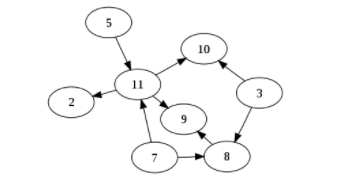
• All the edges are directed.
  Example: Route network

Undirected graph

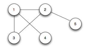
• All the edges are undirected.

          Example: Flight network

Vertices, edges, and degrees

• When an edge connects two vertices, the vertices are said to be adjacent to each other and the edge is incident on both the vertices.
• Two edges are parallel to each other if they connect the same pair of vertices.
• The degree of a vertex represents the number of edges incident on it.

Other terminologies

• A cycle is a path where the first and the last vertices are the same. A simple cycle is a cycle with no repeated vertices or edges.
• A graph with no cycles is called a tree. A tree is an acyclic connected graph.
• A subgraph is a subset of a graph’s edge (with associated vertices) that forms a graph.
• A path in a graph is a sequence of adjacent vertices. A simple path is a path with no repeated vertices.
• A graph is called connected if there is a path from every vertex to every other vertex.
• A directed acyclic graph is a directed graph with no cycles.
• A forest is a disjoint set of trees. 
• A spanning tree of a connected graph is a subgraph that contains all of that graph’s vertices and is also a single tree. 
• A bipartite graph is a type of graph whose vertices can be divided into two sets such that all edges connect to a vertex in one set with the vertex in the other set.
• A graph with all its edges present is called a complete graph.
• A graph with relatively few edges is called a sparse graph.

Application of graphs

• Represents relationships between various components in an electronic circuit
• Used in computer networking

You can represent graphs in various ways. The three basic methods for this are as follows:

1. Adjacency matrix
2. Adjacency list
3. Adjacency set

You can refer to this to learn this in detail.

Depth First Search (DFS)

Before you start learning about DFS, watch Graph with music! 

Let’s consider that you are trapped in a maze. If you want to exit the maze, you must visit each path and each intersection (in the worst case). You are using two colors to mark the intersection that you have already passed. When you find a new intersection, you paint it grey and you continue to go deeper. 

After reaching a dead-end, you have no more unexplored paths from the grey intersection, which is now completed, and you mark it in black color. Thus, this ‘dead-end’ represents either an intersection that you have already marked as grey or black or a path that does not lead to an intersection.

In computer science, these intersections of the maze represent the vertices and the path between these intersections represent the edges of a graph. The process of returning from a ‘dead-end’ is referred to as backtracking. 

Initially, all vertices are marked as unvisited (false). The DFS algorithm starts at vertex u in the graph. 

1. If the edge leads to an already-visited vertex, then backtrack to the current vertex u. 
2. If the edge leads to a vertex that has not been visited, then use that vertex to start processing the required data.
3. This means that the new vertex becomes the current vertex.
4. Follow this process until you reach the ‘dead-end’. At this point, you can start backtracking.

The following code is the implementation of the provided scenario:

Note: Assume that visited[] is a global array.

Breadth First Search (BFS)

1. BFS works level by level. Initially, BFS starts at a given index which is at level 0. 
2. In the first stage, it visits all the vertices at level 1.
3. In the second stage, it visits all the vertices at level 2. These new vertices will be adjacent to the level 1 vertices. 
4. BFS continues this process until all the levels of the graph are complete. 

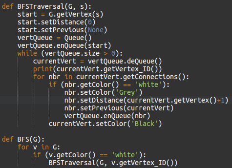
Assume that initially all the vertices are marked unvisited (false). The implementation of the provided scenario is as follows: 

Watch this lecture video on BFS and DFS for better understanding.

Dynamic programming

Dynamic programming is applied to optimization problems. In such problems, there can be many possible solutions. Each solution has a value but you are required to find the solution with the optimal value. 

The development of a dynamic programming-based algorithm can be performed in four steps. They are as follows:

1. Characterize the structure of an optimal solution
2. Recursively define the value of an optimal solution
3. Compute the value of an optimal solution in a bottom-up manner
4. Construct an optimal solution from the computed information

Not all problems can be solved with an optimal solution. To check if you can or not, you can use the following two properties of dynamic programming:

1. Optimal substructure: An optimal solution to a problem contains optimal solutions to subproblems.
2. Overlapping subproblems: A recursive solution contains a small number of distinct subproblems that are repeated multiple times.

Different approaches 

Let’s understand how DP works with an example; the Fibonacci series. 

The recursive implementation of this is as follows:

Here, the complexity is O(2^n).

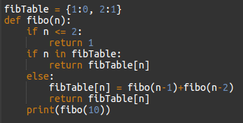
Implementation of the same in top-down approach is as follows:

Implementation of the same in bottom-up approach is as follows:

The two approaches (top-down and bottom-up) of the Fibonacci series reduces the complexity of the program to O(n). This is because, if a value is already computed then you are not required to call the subproblems again. Instead, you are directly taking its value from the table.

Overcall, DP is a very powerful technique to solve a particular class of problems. One easy way to master DP problems is by solving multiple problems. 

TAKE PRACTICE TEST 3

Are you ready to test you Algorithms skills?

The Final Test